Error Propagation
|
Very often we use our physical measurements as a means to some computational end. We may, for example, use measurements of mass and velocity to calculate kinetic energy, or temperature and pressure to calculate molar volume. While we should have a fair grasp on the uncertainty inherent in our physical measurements, we are also interested in bounding the uncertainty in those calculated values. Methods of error propagation allow us to translate the error in independent variables into the error within the dependent variables of our functions.
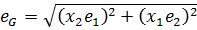
Let's take a very simple example (This example will illustrate the difference of two variables, but the results for error propagation in addition are the same). Say we wanted to know the weight of a liquid in a container. We take the weight of the empty container, w1, then fill it with our liquid and take the weight again, w2. Each weight, w1 and w2, comes with a range of uncertainty, ±e1 and ±e2 respectively (always at some confidence level). In this example, these errors depend on the precision of the scale we used.
Of course, the weight of the liquid, w0, should be the difference, w2 - w1, but what is our uncertainty in w0?
At first glance, we might expect the range of w0 to be between the maximum and minimum values possible if we take our measured weights at their extremes:

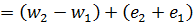

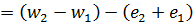
making the uncertainty (error) in w0:
 .
.
However, in reality, this value of e0 is too pessimistic. Think of tossing two six-sided dice and adding the resulting numbers together. With individual die, we have a 1 in 6 chance (16.7%) to get each number, including the extremes of 1 and 6. However, when we add the die together, the numbers at the extremes of that calculated value become less likely. For the extremes in the calculated value of 12 or 2, the probability drops to (1/6)*(1/6)=2.78%, while the mean value of 7 remains at 16.7%.
To illustrate this concept with our liquid weight example, let's assume w1 = 1 g, w2 = 2 g, and the error associated with both measurements is ± 0.1 g. For simplicity and illustration, assume the measurements are normally distributed and the error we are reporting is one standard deviation (This confidence interval is associated with a low confidence level, but the same equations for error propagation are obtained with stricter levels).
Figure 1 shows the result of performing this simulated experiment three times, in the form of three histograms (with weight on the x-axis). Figure 2 shows the normal distributions we obtain from the standard deviations of the data, w1 and w2, and the calculated liquid weight, w0, along with the distribution we would find if e0= e1+e2 (the distributions are all normalized to have zero mean, for comparison purposes).
Figure 1: Histograms. |
Figure 2: Distributions. |
||||||||||
|
|
As you can see, three "experiments" are not sufficient to reach any empirical conclusions about what the propagated error, e0, should be. However, as you perform more and more experiments, you should notice that the distribution of the calculated value of w0 (green) is clearly broader than the distribution of either w1 or w2, but it is not broader than what it would be if e0= e1+e2 = 0.2 (purple). Instead, with more and more experiments, e0 approaches 0.020.5 (0.14142135623731...), or should assuming the random number generator in javascript is up to the task.
The analytical reason for this result is the fact that the sum (or difference) of two normally distributed random variables results in a normal distribution with a variance that is the sum of the variances of the two original distributions (see several proofs here). Therefore, the resulting standard deviation (or any confidence interval) when adding two variables is the square root of the sum of the squares of the original variance. In terms of errors:
![]() .
.
Using Equation 4 we obtain our result for the example above without thousands of simulated experiments: e0 = (0.12 + 0.12)0.5 = 0.020.5 = 0.1414.
Error Propagation for Arbitrary Functions:
Of course, we often deal with mathematical operations more complicated than addition and subtraction. For arbitrary functions of multiple variables we have several options, each with its own strength and weakness.
Analytical Method for Error Propagation:
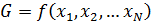
Assume we wish to calculate the value of G, which is a function of variables x1 to xN. We may approximate our function with a 1st order Taylor series and find an equation for the error, eG, as a function of the error in our independent variables, e1 to eN.
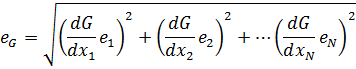
For example, if our function G = x1x2, then:
Numerical Method for Error Propagation:
Alternatively, the linearization may be accomplished numerically. Once again we have a function of N independent variables:
To find the error in G numerically, we first calculate f0, which is G calculated without consideration of error:
Next, for each independent variable, we calculate a fi, which is the function, G, calculated with only variable i equal to its measured value plus its error, and the remaining variables at their mean, or measured value:

Finally we sum the squares of the difference between each fi and f0, and take the square root to find the error in the calculated value of G:
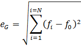
This method also involves an approximation to the function, but it has several advantages. Because there is no need to take partial derivatives, this is a simple method of error propagation to automate for general use. Also, in instances where G is itself calculated numerically, and we cannot obtain analytical partial derivatives, this method remains functional.
Monte Carlo Method for Error Propagation:
Lastly we may use a random number generator in order to find the error in our calculated value, G. This method is the method shown graphically in the liquid weight example in the previous section for the difference of two random variables, but it is broadly applicable to other operations.
For each of our N measured variables, xi, we calculate a random number, xi*, with a normally distributed pdf having a mean of xi and a standard deviation, σ, which is calculated from the variable's confidence interval, ei, and confidence level. For a normal distribution:
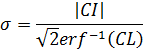
where CI is the confidence interval, or error in our case (ei), and CL is the confidence level, which is typically 95 or 90%.
Note that this random number need not, in actuality, come from a normal distribution--it may be based on any distribution or even empirical data from a histogram--but here we will only present this most common case.
We then calculate G using x1* through xN* in place of x1 through xN, and repeat this step M times, each time calculating a new set of random variables x*, until we've collected a large number of M calculated values of G, G1 through GM. The standard deviation of that set will approach the appropriate propagated error, e0, as M becomes larger.
On the down side, this method is computationally expensive and give no indication on which variables contribute most to the error. However, it may give more accurate results than the other methods discussed here, given a large enough M. For example, note that if your equation is highly nonlinear you may obtain significantly different results for the numerical method by various combinations of adding or subtracting the error from the measured values, all of which are equally valid results. The Monte Carlo method, given enough time, samples through the entirety of all variable-error combinations, and thus may give a more accurate picture of the propagated error. Furthermore, this method give us the ability to use any pdf for our independent variables, instead of simple error values, and, by plotting the values of G1 through GM in a histogram, we may also obtain a detailed pdf of the calculated value, as shown in Figure 1, above.
The following example will show how the methods for error propagation for an arbitrary function, which were discussed in the previous section, may be used on an real-world problem.
Suppose you had a jar of honey and you wished to determine the viscosity, as well as the interval of uncertainty in that value. Without more sophisticated equipment, a quick and simple way to do this would be falling sphere viscometry. In this experiment the terminal velocity of a bead falling through a viscous liquid is measured. Assuming stokes flow, the viscosity of the fluid, μ, may be given by the following equation:
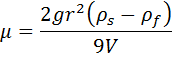
where r is the radius of the sphere, g is the gravitational constant, V is the terminal velocity, and ρs and ρf are the densities of the sphere and the fluid respectively.
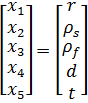
Our first step is to decide what our measurements are. Of the variables in Equation 12, the only one that we directly measure is r. Let us assume that, in a separate set of experiments we determined ρs and ρf and the associated errors. However, as we conduct the falling sphere experiment we do not directly measure terminal velocity; we measure the distance the bead travels, d, over a certain amount of time, t. Thus our vector of measurements, x, should be:
Note that even if we do not know the gravitational constant, g, to infinite precision, we have enough significant figures that we may assume it is not a significant source of error and may be treated as a constant.
For the continuous method of Equations (5) and (6), we must take partial derivatives of Equation (13) with respect to each x. Those derivatives can be seen in blue analytical section of the following table, along with some example values for each variable and its associated error:
|
|||||||||||
| Variables & Error |
Analytical Method |
Numerical Method |
Monte Carlo Method |
||||||||
| i | xi | ei | df / dxi | ( df / dxi ei )2 | fi | ( fi - f0 )2 | M = | ||||
| 0 | -- | -- | -- | -- | ?? | 0 | CL = % | ||||
| 1 | |||||||||||
| 2 | |||||||||||
| 3 | |||||||||||
| 4 | |||||||||||
| 5 | |||||||||||
|
Insert additional variable |
|||||||||||
Sum : |
|||||||||||
f = ?? ± |
|||||||||||
|
|||||||||||
For the analytical method, we calculate values for the derivatives multiplied by the associated error, and square them (as seen in the second column of the blue section above). Using Equation (6), we then take the sum and find our error as the square root of that sum. Thus, for this method, the reported viscosity would be 83 ± 6 g/cm/s.
The numerical method, as described by Equations (9)-(11), is also shown in the table above (red section). We first calculate f0 and then f1 through f5, which are calculated with only variable i equal to its measured value plus its error. We then calculate the square of the difference between fi and f0 for each variable, and sum them. The resulting error is the square root of that sum (6.009 g/cm/s), and the reported viscosity should be 83 ± 6 g/cm/s.
Note that, in the above example, the values in the second columns of both the analytical and numerical sections (blue and red) contain what we call sensitivity coefficients, and their magnitudes indicate their variable's contribution to the error in our calculated value. As can be seen, the greatest contributor to the error in our calculated viscosity is the measurement of our sphere's radius. If we wished to improve our precision, we would find the greatest benefit in improving our radius measurement. To see this effect, reduce the error in the radius measurement by an order of magnitude and you'll see the error diminish and our time measurement then become our greatest concern.
Lastly, the table above shows the results of the Monte Carlo method (yellow section). For each variable, 1,000 values (M) are calculated with a normally distributed random number generator as described above. With those values of x, M values of our function are calculated. The resulting standard deviation of that set of calculated values is then taken as our propagated error. Note that increasing or decreasing the number of experiments, M, can have significant impact on these results. However, with M=1,000, we get very similar results to the other methods: μ = 83 ± 6 g/cm/s.
Additionally, with the Monte Carlo method, we are able to obtain the distribution of the calculated value, as shown in the above histogram (which is created in the same manner as the histogram for w0 shown above in Figure 1). For this example, the results appear to be very near a normal distribution, but this will not always be the case (For example, set x1 to 0.002 and you will end up with a pdf nearer to a log-normal distribution). The above QQ-Plot indicates the normality of f's PDF. The greater the deviation from linearity in the QQ-Plot, the greater the pdf's deviation from normality.
You may use the above interactive example to get a feel for the effects on error propagation of different measurements and errors, using this function or another function of interest. For easier access, this error propagation gadget may also be found here.