University of Utah

Chemical Engineering Department

Random Variables Projects Lab, University of Utah

 

"I, at any rate, am convinced that He does not throw dice."

 

~ Albert Einstein

• Random Variables
  • Discrete Random Variables
  • Continuous Random Variables
  • Mixed Random Variables
• Cumulative Distribution Functions (CDF)
• Probability Density Function (PDF)
• Interactive CDF/PDF Example

Random Variables:

Say you were to take a coin from your pocket and toss it into the air. While it flips through space, what could you possibly say about its future?

 

Will it land heads up? Tails? More than that, how long will it remain in the air? How many times will it bounce? How far from where it first hits the ground will it finally come to rest? For that matter, will it ever hit the ground? Ever come to rest?

 

For some such questions, we can and do settle on answers long before observations; we are pretty sure gravity will hold and the coin will land. But for others we have no choice but to hold judgment and speak in more vague terms, if we wish to say anything useful about the future at all.

 

As scientists, it is, of course, our job to say something useful (or at the very least, authoritative...), while the metaphorical coins of important physical system are still in the air. Heads or tails may even be a matter of life or death. Our coins may be, for example, various possible coolant flow rates or masses of uranium in a nuclear power plant. We care greatly to know what our chances are that we will get whirring turbines instead of a meltdown.

 

To a strict determinist, all such bets were settled long before any coin, metaphorical or not, was ever minted; we simply do not yet know it. If we only knew the forces applied at a coin's toss, its exact distribution of mass, the various minute movements of air in the room... If we knew all that, then we would know that particular coin toss had a 100% chance of landing the way it will land, and zero chance of any other outcome.

 

But we, of course, are often lacking even a mentionable fraction of such knowledge of the world. Furthermore, it seems on exceedingly small scales that strict determinists are absolutely wrong; there is no way to predict when, for example, a uranium atom will split, and if such an event affects the larger world then that macro event is truly unpredictable. Some outcomes truly are up in the air, unsettled until they are part of the past.

 

In order to cope with this reality and to be able to describe the future states of a system in some useful way, we use random variables. A random variable is simply a function that relates each possible physical outcome of a system to some unique, real number. As such there are three sorts of random variables: discrete, continuous and mixed. In the following sections these categories will be briefly discussed and examples will be given.

 

Discrete Random Variables:

Consider our coin toss again. We could have heads or tails as possible outcomes. If we defined a variable, x, as the number of heads in a single toss, then x could possibly be 1 or 0, nothing else. Such a function, x, would be an example of a discrete random variable. Such random variables can only take on discrete values. Other examples would be the possible results of a pregnancy test, or the number of students in a class room.

 

Continuous Random Variables:

Back to the coin toss, what if we wished to describe the distance between where our coin came to rest and where it first hit the ground. That distance, x, would be a continuous random variable because it could take on a infinite number of values within the continuous range of real numbers. The coin could travel 1 cm, or 1.1 cm, or 1.11 cm, or on and on. Other examples of continuous random variables would be the mass of stars in our galaxy, the pH of ocean waters, or the residence time of some analyte in a gas chromatograph.

 

Mixed Random Variables:

Mixed random variables have both discrete and continuous components. Such random variables are infrequently encountered. For a possible example, though, you may be measuring a sample's weight and decide that any weight measured as a negative value will be given a value of 0. In that way the random variable has a discrete component at x = 0 and continuous component where x > 0.

 

Cumulative Distribution Functions (CDF):

The question, of course, arises as to how to best mathematically describe (and visually display) random variables. For those tasks we use probability density functions (PDF) and cumulative density functions (CDF). As CDFs are simpler to comprehend for both discrete and continuous random variables than PDFs, we will first explain CDFs.

 

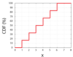
Consider tossing a fair 6-sidded dice. We would have a 1 in 6 chance of getting any of the possible values of the random variable (1, 2, 3, 4, 5, or 6). If we plot those possible values on the x-axis and plot the probability of measuring each specific value, x, or any value less than x on the y-axis, we will have the CDF of the random variable.

 

This function, CDF(x), simply tells us the odds of measuring any value up to and including x. As such, all CDFs must all have these characteristics:

1. A CDF must equal 0 when x = -∞, and approach 1 (or 100%) as x approaches +∞. Simply put, out of all the possible outcomes, there must be an outcome; the chance of tossing a six sided dice and getting a value between -∞ and ∞ is 100%.
2. The slope of a CDF must always be equal to or greater than zero. For example, consider the chance of tossing a 6-sidded dice (fair or not) and obtaining a value between 0 and 4. That chance cannot possibly be more than the chance of obtaining a value between 0 and 5, because the odds of a 1, 2, or 3 landing face up are, of course, always going to be some fraction of the odds of getting a 1, 2, 3, or 4.

For an example of a continuous random variable, the following applet shows the normally distributed CDF.

 

This important distribution is discussed elsewhere. Simply note that the characteristics of a CDF described above and explained for a discrete random variable hold for continuous random variables as well.

 

For more intuitive examples of the properties of CDFs, see the interactive example below. Also, interactive plots of many other CDFs important to the field of statistics and used on this site may be found here.

 

Probability Density Functions (PDF):

A PDF is simply the derivative of a CDF. Thus a PDF is also a function of a random variable, x, and its magnitude will be some indication of the relative likelihood of measuring a particular value. As it is the slope of a CDF, a PDF must always be positive; there are no negative odds for any event. Furthermore and by definition, the area under the curve of a PDF(x) between -∞ and x equals its CDF(x). As such, the area between two values x₁ and x₂ gives the probability of measuring a value within that range.

 

The following applet shows an example of the PDF for a normally distributed random variable, x.

 

 

Notice, when the mean and standard deviations are equal, how the PDF correlates with the normal CDF in the section above.

 

Also consider the difference between a continuous and discrete PDF. While a discrete PDF (such as that shown above for dice) will give you the odds of obtaining a particular outcome, probabilities with continuous PDFs are matters of range, not discrete points. For example, there is clearly a 1 in 6 (16.6%) chance of rolling a 3 on a dice, as can be seen in its PDF. But what are the odd of measuring exactly zero with a random variable having a normal PDF and mean of zero, as shown above? Even though it is the value where the PDF is the greatest, the chance of measuring exactly 0.00000... is, perhaps counter intuitively, zero. The odds of measuring any particular random number out to infinite precision are, in fact, zero.

 

With a continuous PDF you may instead ask what the odds are that you will measure between two values to obtain a probability that is greater than zero. To find this probability we simply use the CDF of our random variable. Because the CDF tells us the odd of measuring a value or anything lower than that value, to find the likelihood of measuring between two values, x₁ and x₂ (where x₁ > x₂), we simply have to take the value of the CDF at x₁ and subtract from it the value of the CDF at x₂. For example, using the normal CDF in the applet above (with μ=0, and σ=1), if we wished to know the odds of measuring between 0.01 and 0.02 we find CDF(x=0.1)=53.9828% and CDF(x=0.2)=57.9260%. Then the difference, CDF(0.2)-CDF(0.1), gives us the odds of about 3.9% of measuring an x between 0.1 and 0.2.

 

For more intuitive, visual examples of the properties of PDFs, see the interactive example below. Also, interactive plots of many important PDFs used on this site may be seen here.

 

Interactive CDF/PDF Example:

 

Select a type of random variable: ~ Discrete ~ Uniform Binomial Arbitrary ~ Continuous ~ Uniform Normal Log-Normal Exponential Student-t Chi-Squared F

show Random variable details:

PDF CDF     Example, Determining Probabilities: Assuming the above PDF, what is the probability that a measurement, x, will be: Above Below Equal To and or Above Below Equal To           Simulated Experiments with the Population Having the Above PDF: